Taiwan Space Agency (TASA) Intern | Winston Wei-Han Chou

Overview

During my two-month internship at Taiwan Space Agency (TASA) under the Space Transportation Avionics division, I contributed to advancing the TAI-namics Software Stack with a primary focus on progressing from Model-in-Loop (MIL) testing toward Hardware-in-Loop (HIL) implementation. My work encompassed software integration, interface optimization, and research into advanced propellant sloshing dynamics modeling.

Research Project

Mechanical Modeling of 3D Propellant Sloshing in Fuel Tanks Using SE(3) Screw Motion Theory

I. Introduction

Accurate modeling of propellant slosh dynamics is essential for safe and reliable design of rockets and launch vehicles, as liquid propellant’s motion significantly affects vehicle stability and control. While Computational Fluid Dynamics (CFD) provides detailed insight into fluid behavior, its high computational cost makes it impractical for rapid simulation and design iteration [5]. This study adopts the equivalent pendulum method [1], [2], [3], but extends its rigor and generality by embedding it within the SE(3) screw motion framework [4]. By expressing both tank motion and slosh-induced wrenches using twist and wrench coordinates, the model naturally handles arbitrary 3D maneuvers. The result is a fast, physically grounded tool for predicting slosh forces and validating against CFD across realistic scenarios.

Why pendulum model: Fast, physically meaningful, captures main slosh resonance, widely used in industry.
Why SE(3): Fully 3D, consistent for coupled rotational/translational dynamics, extensible to more complex motions.
Validation: CFD comparison confirms accuracy for engineering use.

II. Methodology

Figure 1. Equivalent-Pendulum Model

Pendulum parameters are calculated based on tank geometry and liquid properties. [3] The coupled dynamics of the tank and internal pendulum are derived using Lagrangian mechanics, with states represented as pose, twist, and relative twist. $$\,^{\mathcal{B}}T_{\mathcal{H_{\text{i}}}} \in SE(3), \,^{\mathcal{B}}\mathcal{V}_{\mathcal{B}}^{\wedge} \in \mathfrak{se}(3), \,^{\mathcal{H_{\text{i}}}}\mathcal{V}_{\mathcal{H_{\text{i}}}/\mathcal{B}}^{\wedge} \in \mathfrak{se}(3)$$ Lagrangian Formulation: \begin{align} \mathcal{L} &= \frac{1}{2} {\,^{\mathcal{B}}\mathcal{V}_{\mathcal{B}}}^\top \,^{\mathcal{B}}\mathcal{G}_{\mathcal{B}} \,^{\mathcal{B}}\mathcal{V}_{\mathcal{B}} + \frac{1}{2} {\,^{\text{0}}\mathcal{V}_{\text{0}}}^\top \,^{\text{0}}\mathcal{G}_{\text{0}} \,^{\text{0}}\mathcal{V}_{\text{0}} + \frac{1}{2} \sum_{i=1}^{n} {\,^{\mathcal{P_{\text{i}}}}\mathcal{V}_{\mathcal{P_{\text{i}}}}}^\top \,^{\mathcal{P_{\text{i}}}}\mathcal{G}_{\mathcal{P_{\text{i}}}} \,^{\mathcal{P_{\text{i}}}}\mathcal{V}_{\mathcal{P_{\text{i}}}} \label{eq:test1} \\ \delta \mathcal{L} &= \frac{\delta \mathcal{L}}{\delta \,^{\mathcal{B}}\mathcal{V}_{\mathcal{B}}} \delta \,^{\mathcal{B}}\mathcal{V}_{\mathcal{B}} + \sum_{i=1}^{n} \frac{\delta \mathcal{L}}{\delta \,^{\mathcal{H_{\text{i}}}}\mathcal{V}_{\mathcal{H_{\text{i}}}/\mathcal{B}}} \delta \,^{\mathcal{H_{\text{i}}}}\mathcal{V}_{\mathcal{H_{\text{i}}}/\mathcal{B}} + \frac{\delta \mathcal{L}}{\delta \,^{\mathcal{B}}{\mathcal{T}}_{\mathcal{H_{\text{i}}}}} \delta \,^{\mathcal{B}}{\mathcal{T}}_{\mathcal{H_{\text{i}}}} \end{align} Principle of Stationary Action: \begin{align} \delta \mathcal{A} = \int_{t_1}^{t_2} \delta \mathcal{L} \left(\,^{\mathcal{B}}\mathcal{V}_{\mathcal{B}}, \,^{\mathcal{H_{\text{i}}}}\mathcal{V}_{\mathcal{H_{\text{i}}}/\mathcal{B}}, \,^{\mathcal{B}}{\mathcal{T}}_{\mathcal{H_{\text{i}}}} \right) = 0 \label{eq:PofSA} \end{align}

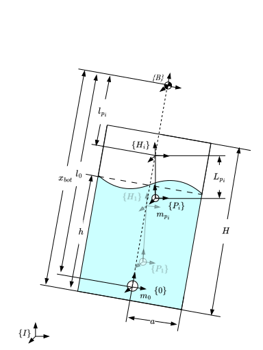
According to the Principle of Stationary Action, solving Eq. \eqref{eq:PofSA} leads to Equation of Motions (EoMs) of the equivalent-pedulum model in SE(3).

Equation of Motions: \(\begin{align} &\begin{cases} \begin{aligned} &\,^{\mathcal{B}}{\mathcal{G}}_{\mathcal{B}} \,^{\mathcal{B}}{\mathcal{\dot V}}_{\mathcal{B}} - {\,^{\mathcal{B}}{\mathcal{V}}_{\mathcal{B}}^{\curlywedge}}^\top \,^{\mathcal{B}}{\mathcal{G}}_{\mathcal{B}} {\,^{\mathcal{B}}{\mathcal{V}}_{\mathcal{B}}} + \,^{\mathcal{B}}{\mathcal{T}}_{\mathcal{\text{0}}}^{-\top} \left( \,^{\text{0}}{\mathcal{G}}_{\text{0}} \,^{\text{0}}{\mathcal{\dot V}}_{\text{0}} - {\,^{\text{0}}{\mathcal{V}}_{\text{0}}^{\curlywedge}}^\top \,^{\text{0}}{\mathcal{G}}_{\text{0}} \,^{\text{0}}{\mathcal{V}}_{\text{0}}\right) \\ &\quad + \sum_{i=1}^{n} \Bigg[ \,^{\mathcal{B}}{\mathcal{T}}_{\mathcal{H_{\text{i}}}}^{-\top} \left( \,^{\mathcal{H_{\text{i}}}}{\mathcal{T}}_{\mathcal{P_{\text{i}}}}^{-\top} \,^{\mathcal{P_{\text{i}}}}{\mathcal{G}}_{\mathcal{P_{\text{i}}}} \,^{\mathcal{P_{\text{i}}}}{\mathcal{\dot V}}_{\mathcal{P_{\text{i}}}} + {\,^{\mathcal{H_{\text{i}}}}{\mathcal{V}}_{\mathcal{H_{\text{i}}} / \mathcal{B}}^{\curlywedge}}^\top \,^{\mathcal{H_{\text{i}}}}{\mathcal{T}}_{\mathcal{P_{\text{i}}}}^{-\top} \,^{\mathcal{P_{\text{i}}}}{\mathcal{G}}_{\mathcal{P_{\text{i}}}} \,^{\mathcal{P_{\text{i}}}}{\mathcal{V}}_{\mathcal{P_{\text{i}}}}\right) \\ &\quad\quad\quad\quad - {\,^{\mathcal{B}}{\mathcal{V}}_{\mathcal{B}}^{\curlywedge}}^\top \,^{\mathcal{B}}{\mathcal{T}}_{\mathcal{H_{\text{i}}}}^{-\top} \,^{\mathcal{H_{\text{i}}}}{\mathcal{T}}_{\mathcal{P_{\text{i}}}}^{-\top} \,^{\mathcal{P_{\text{i}}}}{\mathcal{G}}_{\mathcal{P_{\text{i}}}} \,^{\mathcal{P_{\text{i}}}}{\mathcal{V}}_{\mathcal{P_{\text{i}}}} \Bigg] &= \,^{\mathcal{B}}{\mathcal{F}}_\mathcal{B} \\ &\,^{\mathcal{H_{\text{i}}}}{\mathcal{T}}_{\mathcal{P_{\text{i}}}}^{-\top} \,^{\mathcal{P_{\text{i}}}}{\mathcal{G}}_{\mathcal{P_{\text{i}}}} \,^{\mathcal{P_{\text{i}}}}{\mathcal{\dot V}}_{\mathcal{P_{\text{i}}}} \\ &\quad - \left( {\,^{\mathcal{H_{\text{i}}}}{\mathcal{V}}_{\mathcal{H_{\text{i}}} / \mathcal{B}}^{\curlywedge}}^\top + \,^{\mathcal{B}}{\mathcal{T}}_{\mathcal{H_{\text{i}}}}^\top {\,^{\mathcal{B}}{\mathcal{V}}_{\mathcal{B}}^{\curlywedge}}^\top \,^{\mathcal{B}}{\mathcal{T}}_{\mathcal{H_{\text{i}}}}^{-\top}\right) \,^{\mathcal{H_{\text{i}}}}{\mathcal{T}}_{\mathcal{P_{\text{i}}}}^{-\top} \,^{\mathcal{P_{\text{i}}}}{\mathcal{G}}_{\mathcal{P_{\text{i}}}} \,^{\mathcal{P_{\text{i}}}}{\mathcal{V}}_{\mathcal{P_{\text{i}}}} , \quad\quad \forall \{i=1\text{ to }n\} &= 0 \label{eq:SE3_pendulum_eoms} \end{aligned} \end{cases} \\\nonumber\\ &\,^{\text{0}}{\mathcal{V}}_{\text{0}} = \,^{\mathcal{B}}{\mathcal{T}}_{\mathcal{\text{0}}}^{-1} \,^{\mathcal{B}}{\mathcal{V}}_{\mathcal{B}} \nonumber \\ &\,^{\mathcal{P_{\text{i}}}}{\mathcal{V}}_{\mathcal{P_{\text{i}}}} = \,^{\mathcal{H_{\text{i}}}}{\mathcal{T}}_{\mathcal{P_{\text{i}}}}^{-1} \left( \,^{\mathcal{B}}{\mathcal{T}}_{\mathcal{H_{\text{i}}}}^{-1} \,^{\mathcal{B}}{\mathcal{V}}_{\mathcal{B}} + \,^{\mathcal{H_{\text{i}}}}{\mathcal{V}}_{\mathcal{H_{\text{i}}} / \mathcal{B}}\right) \nonumber \\ &\,^{\text{0}}{\mathcal{\dot V}}_{\text{0}} = \,^{\mathcal{B}}{\mathcal{T}}_{\mathcal{\text{0}}}^{-1} \,^{\mathcal{B}}{\mathcal{\dot V}}_{\mathcal{B}} \nonumber \\ &\,^{\mathcal{P_{\text{i}}}}{\mathcal{\dot V}}_{\mathcal{P_{\text{i}}}} = \,^{\mathcal{H_{\text{i}}}}{\mathcal{T}}_{\mathcal{P_{\text{i}}}}^{-1} \left( \,^{\mathcal{B}}{\mathcal{T}}_{\mathcal{H_{\text{i}}}}^{-1} \,^{\mathcal{B}}{\mathcal{\dot V}}_{\mathcal{B}} + \,^{\mathcal{H_{\text{i}}}}{\mathcal{\dot V}}_{\mathcal{H_{\text{i}}} / \mathcal{B}} + \,^{\mathcal{B}}{\mathcal{T}}_{\mathcal{H_{\text{i}}}}^{-1} {\,^{\mathcal{B}}{\mathcal{V}}_{\mathcal{B}}^{\curlywedge}} \,^{\mathcal{B}}{\mathcal{T}}_{\mathcal{H_{\text{i}}}} \,^{\mathcal{H_{\text{i}}}}{\mathcal{V}}_{\mathcal{H_{\text{i}}} / \mathcal{B}}\right) \end{align}\)

Where $\mathcal{T}=\text{Ad}(T)$ is the Adjoint map of $SE(3)$, and $\mathcal{V}^{\curlywedge}=\text{ad}(\mathcal{V})$ is the adjoint map of $\mathfrak{se}(3)$:

\[\begin{align} \,^{\mathcal{B}}{\mathcal{T}}_{\mathcal{H_{\text{i}}}} &= \text{Ad}[\,^{\mathcal{B}}T_{\mathcal{H_{\text{i}}}}] = \text{Ad}_{\,^{\mathcal{B}}T_{\mathcal{H_{\text{i}}}}} \\ \,^{\mathcal{B}}{\mathcal{V}}_{\mathcal{B}}^{\curlywedge} &= \text{ad}[\,^{\mathcal{B}}{\mathcal{V}}_{\mathcal{B}}] = \text{ad}_{\,^{\mathcal{B}}{\mathcal{V}}_{\mathcal{B}}} \\ \,^{\mathcal{H_{\text{i}}}}{\mathcal{V}}_{\mathcal{H_{\text{i}}} / \mathcal{B}}^{\curlywedge} &= \text{ad}[\,^{\mathcal{H_{\text{i}}}}{\mathcal{V}}_{\mathcal{H_{\text{i}}} / \mathcal{B}}] = \text{ad}_{\,^{\mathcal{H_{\text{i}}}}{\mathcal{V}}_{\mathcal{H_{\text{i}}} / \mathcal{B}}} \end{align}\]

III. Results

Figure 2. At a simulation time step of 0.004 sec, the comparison of propellant slosh side force simulations under four applied lateral acceleration test cases (see Table 1 for input profile details). For each case (columns 1–4), the top row displays the time history of side force on the tank wall computed by CFD simulation (blue), standard 2nd-order linear ODE model (red), and the proposed SE(3)-based model (green). The middle row shows the pointwise force differences between the two reduced models and the CFD results. The bottom row presents the corresponding side force frequency spectra from Fourier analysis, highlighting the predicted and observed dominant slosh modes.

IV. Conclusions

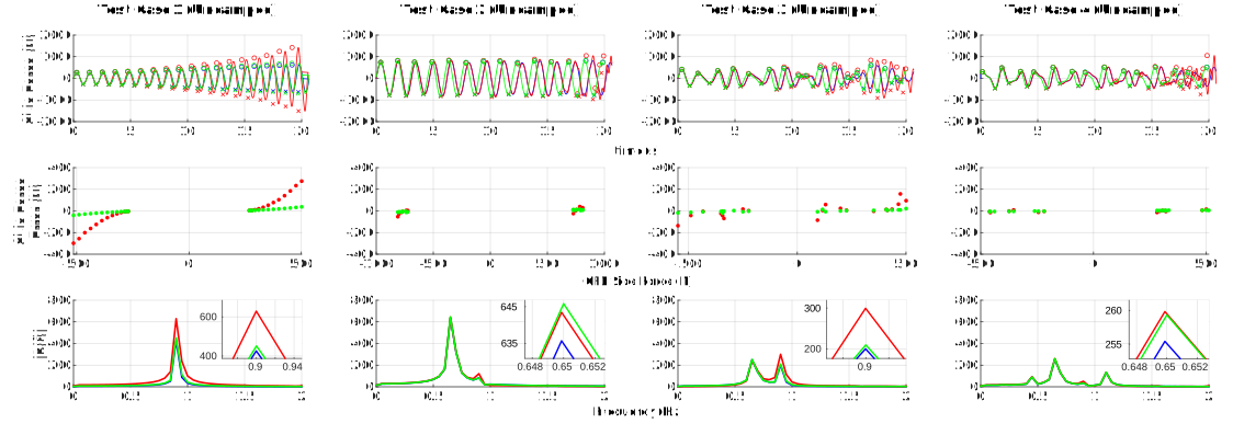
This study derives and validates the SE(3)-based equivalent pendulum slosh model, demonstrating that it recovers standard 2D results [1], [2] when reduced to planar motion, thus confirming its effectiveness as a 3D extension of the equivalent pendulum approach.
Application of Lagrangian mechanics in the SE(3) framework allows the kinetic energy to be naturally decomposed into a sum of mass-acceleration products for each pendulum, yielding deeper physical insight into coupled slosh dynamics.
The SE(3)-based model retains essential nonlinear terms absent in the conventional linearized 2nd-order ODE formulation. These terms impart intrinsic damping and enhance stability, accurately capturing slosh behavior and avoiding the conditional instability seen in linear models under oscillatory input.
At larger pendulum angles, the SE(3)-based model closely reproduces the qualitative force signatures predicted by high-fidelity CFD, demonstrating its improved fidelity for sloshing dynamics. Future work will explore the model’s validity limits and extend it to account for fluid viscosity and dissipation effects

Technical Skills Developed

Software Engineering

MATLAB-C++ interfacing using MEX framework and libmexclass
Performance optimization and computational bottleneck resolution
Configuration management system implementation
Version control and collaborative development practices

Aerospace Simulation

Spacecraft dynamics modeling in SE(3) framework
Multi-physics system integration (structural, fluid, control systems)
Real-time simulation optimization for MIL-to-HIL progression
Computational fluid dynamics validation methodologies

Research and Analysis

Advanced mathematical modeling using Lie group theory
Lagrangian mechanics application to coupled systems
Technical documentation and research paper preparation
Literature review and comparative analysis skills

Acknowledgement

I am deeply grateful to my mentor, Yen-Cheng Chu, for his guidance and support during this internship, and to my colleagues in the Space Transportation Avionics division for their collaborative efforts and shared expertise. Special thanks to Dr. Wu for creating such an enriching internship experience that allowed me to make meaningful contributions to Taiwan’s space technology initiatives.

References:

[1] C. H. Kim, Commercial Satellite Launch Vehicle Attitude Control Systems Design and Analysis: H-Infinity, Loop Shaping, and Coprime Factorization Approach. CHK, 2007.
[2] H. Marbach, “Analysis and design of space vehicle flight control systems,” in IEEE Transactions on Automatic Control, vol. 19, no. 1, pp. 96-97, February 1974, doi: 10.1109/TAC.1974.1100453.
[3] Roberts, James R., Eduardo R. Basurto, and Pei-Ying Chen. Slosh design handbook I. Vol. 1. National Aeronautics and Space Administration, 1966.
[4] K. Lynch and F. C. Park, Modern Robotics: Mechanics, Planning, and Control. Cambridge, UK: Cambridge University Press, 2017.
[5] Dodge, Franklin T. The new” dynamic behavior of liquids in moving containers”. San Antonio, TX: Southwest Research Inst., 2000.